Inflation Forecasting (Under validation)

Factor Augmented VAR for Inflation Forecasting in Python

Model, variable choice and variable transformation based on Bernanke (2005).

FAVAR

A Factor-Augmented Vector Autoregression (FAVAR) extends the traditional VAR model by incorporating latent factors that summarize information from a large dataset. Standard VAR models are limited by the small number of observed macroeconomic variables, which can lead to omitted variable bias. Bernanke, Boivin, and Eliasz (2005) introduced FAVAR to improve macroeconomic analysis, particularly in monetary policy studies. The model extracts unobserved factors from a large panel of economic indicators using techniques like Principal Component Analysis (PCA) or Kalman filtering, thus enhancing the information set available for forecasting and impulse response analysis.

First, a factor equation represents a large set of observed macroeconomic variables \(X_t\) as a function of latent factors \(F_t\) and a factor loading matrix \(\Lambda\), given by:

\[ X_t = \Lambda F_t + u_t. \]

Second, the VAR structure models the dynamic relationship between factors and a subset of observed macroeconomic variables \(Y_t\), following: \[ \begin{bmatrix} F_t \\ Y_t \end{bmatrix} = A_1 \begin{bmatrix} F_{t-1} \\ Y_{t-1} \end{bmatrix} + \dots + A_p \begin{bmatrix} F_{t-p} \\ Y_{t-p} \end{bmatrix} + \varepsilon_t. \] Here, \(A_i\) are coefficient matrices and \(\varepsilon_t\) is the error term. This structure enables a richer characterization of macroeconomic shocks and policy effects.

We base the excercise on the mentioned paper, particulary variable characterization in either fast or slow variables.

#from Functions import *
from scipy.interpolate import interp1d
import numpy as np
import matplotlib.pyplot as plt
import pandas as pd
import os
from datetime import datetime
import tkinter.filedialog
from datetime import timedelta
import math 
import time
import calendar
from numba import jit
from sklearn.metrics import mean_squared_error
from statsmodels.tsa.api import VAR
import scipy
import statsmodels.tsa.stattools as ts
import statsmodels.tsa as tsa
import matplotlib.pyplot as plt
import numpy as np
import sklearn
from sklearn.metrics import mean_squared_error, r2_score
import statsmodels.api as sm
from datetime import datetime,timedelta
from statsmodels.tsa.stattools import adfuller
from numpy.linalg import cholesky

def Factor(Y, X_slow, n_factors, X_fast='None'):
    #n_time = len(Y.index)
    n_var = len(Y.columns)
    if isinstance(X_fast,str)==True:
        hist = Y.join(X_slow)
    else:
        hist = Y.join(X_slow).join(X_fast)
    
    hist=hist.dropna(axis=0,how='any')

    "step 1 - PCA on all observable variables"
    x = np.mat(hist - hist.mean())
    z = np.mat((hist - hist.mean())/hist.std())
    D, V, S = calculate_pca(hist, n_factors + n_var)
    Psi = np.mat(np.diag(np.diag(S - V.dot(D).dot(V.T))))
    factors = V.T.dot(z.T).T
    C = pd.DataFrame(data=factors, index=hist.index, columns=['C' + str(i+1) for i in range(n_factors+n_var)])
    Loadings_C = calculate_factor_loadings(hist, C)
    
    "step 2 - PCA on slow moving variables"
    x = np.mat(X_slow-X_slow.mean())
    z = np.mat((X_slow-X_slow.mean())/X_slow.std())
    D, V, S = calculate_pca(X_slow, n_factors)
    Psi = np.mat(np.diag(np.diag(S - V.dot(D).dot(V.T))))
    factors = V.T.dot(z.T).T
    F_minus = pd.DataFrame(data=factors, index=X_slow.index, columns=['F_minus' + str(i+1) for i in range(n_factors)])
    Loadings_F_slow = calculate_factor_loadings(X_slow, F_minus)
    
    "step 3 - C_t = b1*Y_t + b2*F_t"
    X = Y.join(F_minus)
    B = calculate_factor_loadings(C, X)
    Lambda_y, Lambda_f = B[:,0:n_var], B[:,n_var:]
    # F_t= Lambda_f^-1*(C_t-Lambda_y*Y_t)
    F = Lambda_f.I.dot((np.mat(C).T - Lambda_y.dot(Y.T))).T
    F = pd.DataFrame(data=F, index=X_slow.index, columns=['F' + str(i+1) for i in range(n_factors)])

    return FactorResultsWrapper(C=C, Lambda_c=Loadings_C, F_minus=F_minus, F=F)
    
class FactorResultsWrapper():
    def __init__(self, C, Lambda_c, F_minus, F):
        self.C = C
        self.Lambda_c = Lambda_c
        self.F_minus = F_minus
        self.F = F

def FAVAR(Factor, Y, lag):
    hist = Y.join(Factor)
    model=VAR(hist,missing='drop').fit(lag,trend='n')
 
    return FAVARResultsWrapper(VAR=model)
    
class FAVARResultsWrapper():
    def __init__(self, VAR):
        self.VAR = VAR
    
    def summary(self):
        print(self.VAR.summary())
        return
    
    def predict(self, Factor, Y, step, freq='M', alpha=0.05):
        hist = Y.join(Factor)
        [forecast_mean,forecast_low,forecast_up] = self.VAR.forecast_interval(hist.values, step, alpha)
        mean = np.concatenate((hist.values, forecast_mean), axis=0)
        up = np.concatenate((hist.values, forecast_up), axis=0)
        low = np.concatenate((hist.values, forecast_low), axis=0)
        
        
        dates = pd.date_range(Y.index[0], periods=len(Y.index)+step,freq=freq)
        
        mean = pd.DataFrame(data=mean[:,0:len(Y.columns)], columns=Y.columns.tolist(), index=dates)
        low = pd.DataFrame(data=low[:,0:len(Y.columns)], columns=Y.columns.tolist(), index=dates)
        up = pd.DataFrame(data=up[:,0:len(Y.columns)], columns=Y.columns.tolist(), index=dates)
        
        return [mean,low,up]
    
    def predict_plot(self, Factor, Y, step, freq='M', alpha=0.05, figure_size=[18,12],line_width=3.0,font_size='xx-large', actural='None'):
        mean, low, up = self.predict(Factor, Y, step, freq, alpha)
        n_var = len(mean.columns)
        n_act = len(Y.index)
        
        plt.rcParams['figure.figsize'] = (figure_size[0], figure_size[1])
        plt.rcParams['lines.markersize'] = 6
        plt.rcParams['image.cmap'] = 'gray'
        
        for i in range(n_var):
            plt.figure()
            plt.plot(mean.index[n_act-1:],mean.iloc[n_act-1:,i],color='r',label='forecast', linewidth=line_width)
            plt.plot(mean.index[:n_act],mean.iloc[:n_act,i],color='k',label='observed',linewidth=line_width)
            plt.plot(mean.index[n_act-1:],low.iloc[n_act-1:,i],color='r', linestyle = '--', label='lower - '+str(int(100-alpha*100))+'%',linewidth=line_width)
            plt.plot(mean.index[n_act-1:],up.iloc[n_act-1:,i],color='r', linestyle = ':', label='upper - '+str(int(100-alpha*100))+'%',linewidth=line_width)
            plt.legend()
            if isinstance(actural,str)!=True:
                plt.plot(mean.index[n_act-1:],actural.iloc[:,i],color='k',label='observed', linewidth=line_width)
            plt.title(mean.columns[i], fontweight='bold', fontsize=font_size)
            #plt.xlabel('Date')
            #plt.ylabel('Value')
            plt.show()
        
        return

#from FactorAugmentedVAR import *
#from Functions import *
from datetime import *
import warnings
import pandas as pd
warnings.filterwarnings('ignore')

# Data Import
file_name ='favardata.xlsx'
sheet_name ='Sheet1'
Temp = pd.read_excel(file_name, sheet_name)
vintage_transformed = Temp.iloc[:,1:]
vintage_transformed.index = Temp.iloc[:,0]

#Data Interpolation
vintage_intrpl = DataInterpolation(vintage_transformed[1:], 0, len(vintage_transformed.index), 'slinear').dropna(axis=0,how='any')

# Factor Calculation
factor = Factor(Y=pd.DataFrame(vintage_intrpl.iloc[:,0]), 
                X_slow=vintage_intrpl.iloc[:,1:54], 
                n_factors=3, 
                X_fast=vintage_intrpl.iloc[:,54:])

#factor.C.plot()
#factor.F.plot()

favar = FAVAR(Factor=factor.F, Y=pd.DataFrame(vintage_intrpl.iloc[:,0]), lag=12)
#favar.VAR.summary()

mean, low, up = favar.predict(Factor=factor.F[-12:], Y=pd.DataFrame(vintage_intrpl.iloc[-12:,0]), step=24)

favar.predict_plot(Factor=factor.F[-12:], Y=pd.DataFrame(vintage_intrpl.iloc[-50:,0]), step=24, freq='M', alpha=0.8, figure_size=[10,6],line_width=3.0,font_size='xx-large', actural='None')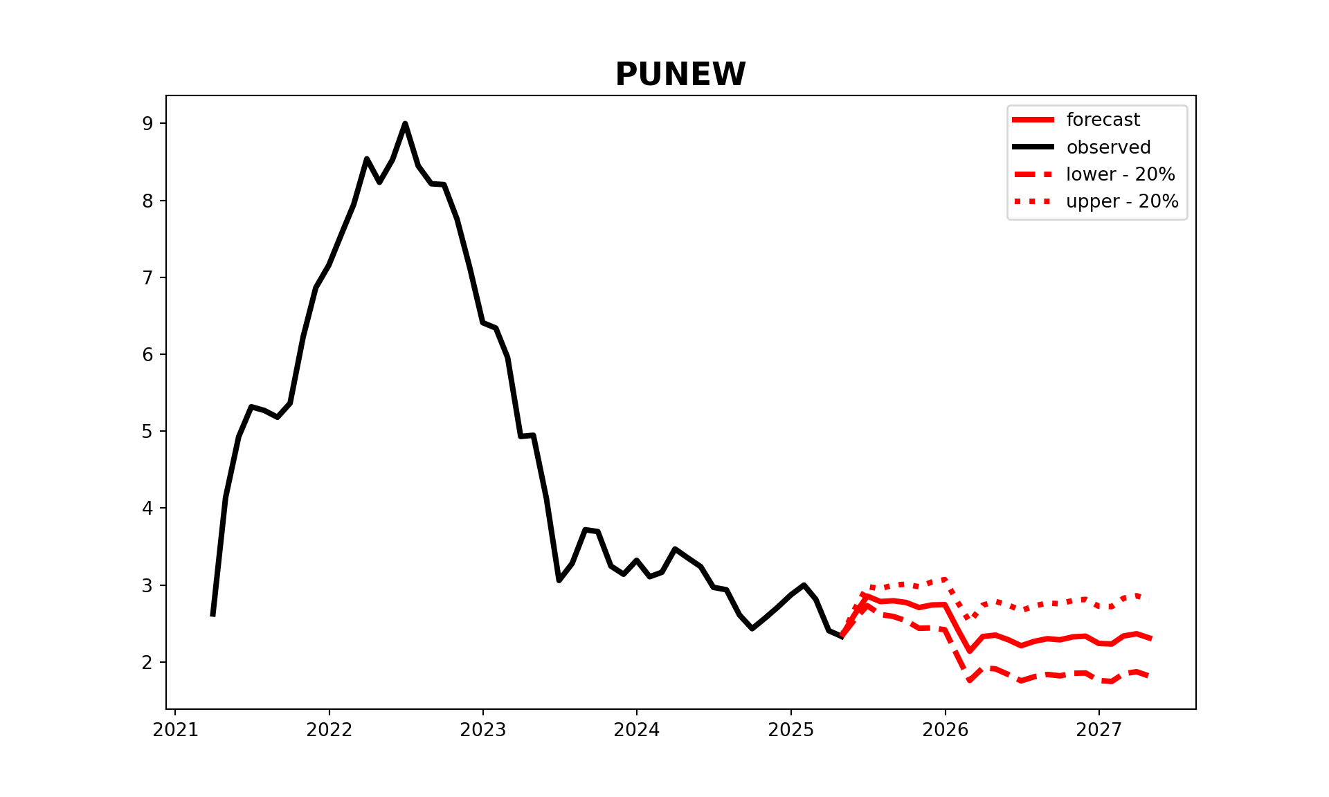

Without differencing between slow/fast variables (k = 3)

slowvars <- reduce(dataframes_list, full_join, by = "date")
df <- full_join(slowvars, vars, by = "date")
df <- drop_na(df)

X <- df %>% dplyr::select(-date, -PUNEW)
Y <- df %>% dplyr::select(PUNEW) 
K <- 3
h <- 25


X <- as.matrix(X)
Y <- as.matrix(Y)


fore_FAVAR <- function(X, Y, K, y_name, h, y=Y[,y_name], use_VAR = F){
  library("tidyverse")
  library("forecast")
  library("vars")
  library("lmtest")
  
  start <- start(X)
  frequency <- frequency(X)
  X = X[1:length(y),]
  Y = Y[1:length(y),,drop=FALSE]
  
  N = dim(X)[2]
  M = dim(Y)[2]
  T = dim(X)[1]
  
  # extract PC from X
  XtX = t(X) %*% X
  spectral_decomposition <- eigen(XtX)
  eig_vec <- spectral_decomposition$vectors
  eig_val <- spectral_decomposition$values
  
  lam <- 1/sqrt(N) * eig_vec[,(1:K)]
  Fr <- data.matrix(X) %*% lam
  
  # FAVAR with clean factors
  if(use_VAR == F){
    Y_for_VAR = cbind(Fr, Y)
    factor_names = paste('factor', 1:K)
    colnames(Y_for_VAR)[1:K] <- factor_names
  }
  else
    Y_for_VAR = Y
  
  Y_for_VAR <- ts(Y_for_VAR, start = start, frequency = frequency)
  VARselect(Y_for_VAR)
  p = VARselect(Y_for_VAR)$selection[1] # according AIC 
  
  var <- VAR(Y_for_VAR, p)
  y_hat <- forecast::forecast(var, h=h)
  return(y_hat)
}

test <- fore_FAVAR(X = X, Y = Y, K = K, h = h)
test$forecast$PUNEW[3]

$mean
Time Series:
Start = 391 
End = 415 
Frequency = 1 
 [1] 2.912215 2.760476 2.667418 2.508745 2.306481 2.233401 2.152444 2.064320
 [9] 2.021029 1.991098 1.953628 1.943925 1.945302 1.955633 1.976103 2.006338
[17] 2.046984 2.091356 2.134203 2.178510 2.220966 2.262351 2.305349 2.348100
[25] 2.389324