library(dplyr)
library(lmtest)
library(sandwich)
library(ggplot2)
library(fredr)
library(plotly)
library(zoo)LP Replication II
Simple replications of some Local Projections
Figure 5 of Local Projections: Jordà and Taylor (2024)
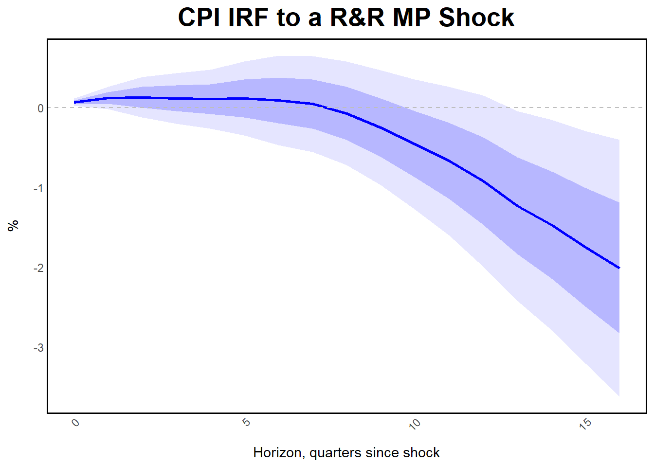
Another simple LP replication: this time, CPI Headline Inflation to a Romer&Romer shock whilst controlling by GDP and FedFunds
data <- haven::read_dta("aggregatedata_final.dta")

data <- data %>%
  mutate(lcpi = 100 * lcpi,
         lrgdp = 100 * lrgdp)

h <- 16
y <- "lcpi"  # Response variable
z <- "rr_shock"  # Instrument variable
nwlag <- h  # N. of Newey-West lags
p <- 0.05  # Significance level


for (i in 0:h) {
  data <- data %>%
    mutate(!!paste0(y, "_f", i) := lead(!!sym(y), i) - lag(!!sym(y), 1))
  }

results <- data.frame(
  horizon = 0:h,
  b = rep(NA, h + 1),
  se = rep(NA, h + 1)
)

# LP Regressions
for (i in 0:h) {
  formula <- as.formula(paste0(
    y, "_f", i, " ~ ", z,
    " + lag(dlrgdp, 1) + lag(dlrgdp, 2) + lag(dlrgdp, 3) + lag(dlrgdp, 4) ",
    " + lag(dlcpi, 1) + lag(dlcpi, 2) + lag(dlcpi, 3) + lag(dlcpi, 4) ",
    " + lag(stir, 1) + lag(stir, 2) + lag(stir, 3)+ lag(stir, 4)"))
  model <- lm(formula, data = data)
  nw_se <- coeftest(model, vcov = NeweyWest(model, lag = h, prewhite = FALSE))

  results$b[i + 1] <- coef(model)[z]
  results$se[i + 1] <- nw_se[z, 2]
  }


results <- results %>%
  mutate(
    u1 = b + se,
    d1 = b - se,
    u2 = b + qnorm(1 - p / 2) * se,
    d2 = b - qnorm(1 - p / 2) * se
    )


ggplot(results, aes(x = horizon)) +
  geom_ribbon(aes(ymin = d2, ymax = u2), fill = "blue", alpha = 0.1) +  # 95% confidence band
  geom_ribbon(aes(ymin = d1, ymax = u1), fill = "blue", alpha = 0.2) +  # Standard error band
  geom_line(aes(y = b), color = "blue", size = 1) +  # Point estimate
  geom_hline(yintercept = 0, linetype = "dashed", color = "gray") +  # Zero line
  labs(x = "Horizon, quarters since shock", y = "%", title = "CPI IRF to a R&R MP Shock") +
theme_minimal() +
     theme(
    plot.title = element_text(hjust = 0.5, size = 20, face = "bold"),
    plot.subtitle = element_text(hjust = 0.5, size = 14, face = "italic", margin = margin(t = 10, b = 10)),
    axis.text.x = element_text(angle = 45, hjust = 1),
    panel.grid.major = element_blank(),
    panel.grid.minor = element_blank(),
    panel.border = element_rect(color = "black", fill = NA, size = 1),
    axis.line = element_blank(),
    axis.ticks.length = unit(-0.25, "cm"),
    axis.title.x = element_text(margin = margin(t = 10)),
    axis.title.y = element_text(margin = margin(r = 10)),
    legend.position = "top",
    legend.title = element_blank(),
    legend.text = element_text(size = 12)
  )
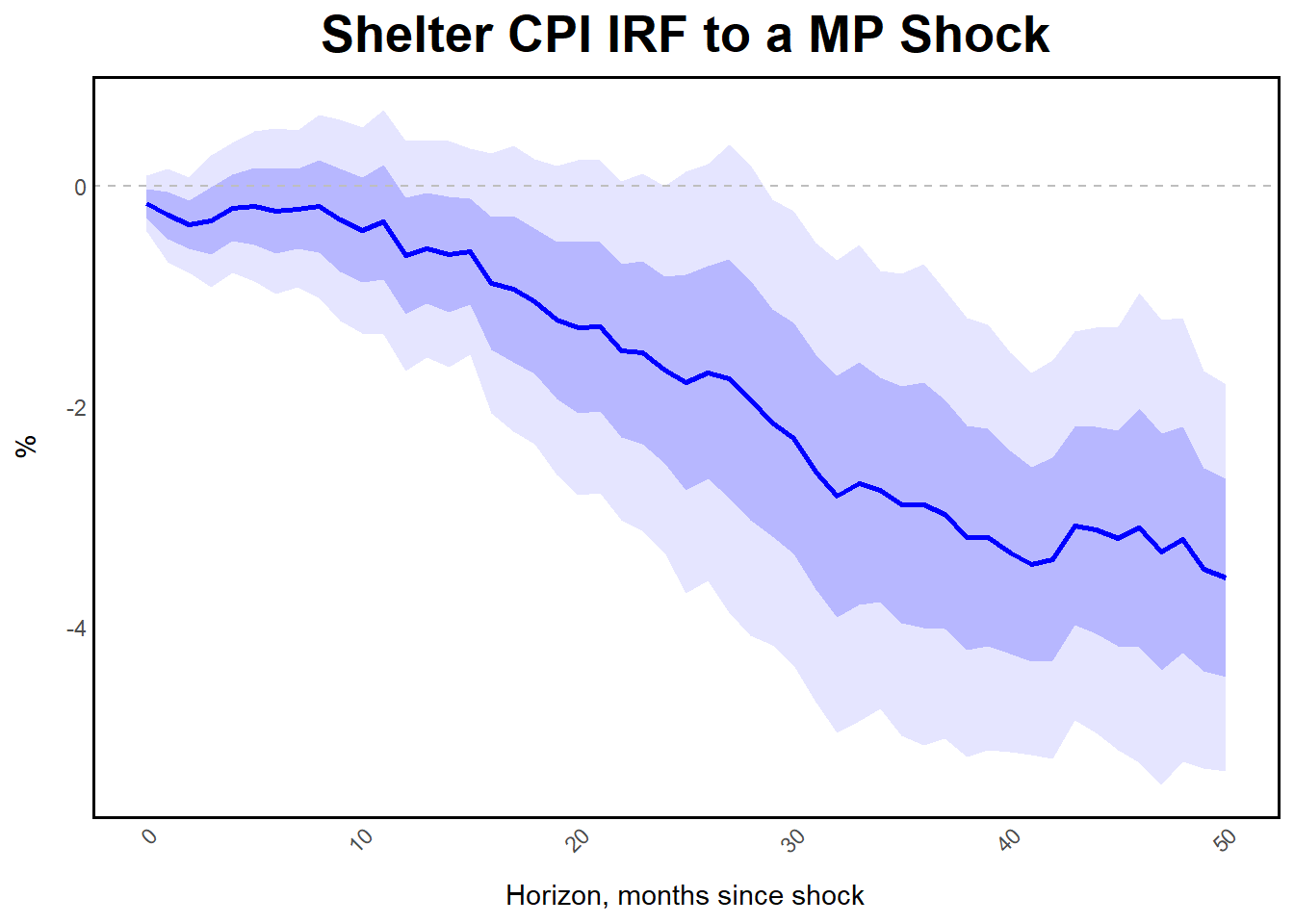
Replication of Figure 4 in Jordà (2024).
The figure illustrates the cumulative impulse response of shelter inflation (measured via the CPI) to a monetary policy shock, identified using high-frequency data from Bauer and Swanson (2023). Paper originally uses PCE inflation, although results are qualitatively similar. The shock isolates monetary policy changes while controlling for information effects. Traditional point-wise confidence intervals (Newey-West adjusted) as shaded bands are used.
Data
key <- "c27bf13d09598a184acdcb2ba94aa28f"
fredr_set_key(key)

cpi <- fredr_series_observations(series_id = "CUSR0000SAH1",
                                 observation_start = as.Date("1969-01-31"),
                                 observation_end = as.Date("2020-3-31"),
                                 frequency = "m",
                                 aggregation_method = "sum",
                                 units = "lin")
cpi <- cpi %>%
  rename(cpi = value) %>%
  mutate(lcpi =log(cpi)) %>%
  select(-series_id, -realtime_start, -realtime_end, -cpi, -date)

data <- haven::read_dta("sigband_shelterinf.dta")
data <- cbind(data, cpi)

data <- data %>%
  dplyr::select(-mon_shock) %>%
  rename(mon_shock = BSmonshock) %>%
  filter(!is.na(mon_shock))
Local Projection
Regress long-difference Shelter CPI with 12 lags of log CPI shelter, unemployment rate and federal funds rate.
# Set parameters
h <- 50 # Plot horizon
p <- 0.05 # Significance level of test
nwlag <- h # Newey-West lags

data <- data %>%
  mutate(lpcepi_house = 100 * lpcepi_house) %>%
  mutate(lcpi = 100*lcpi)

# Generate forward variables for LP regressions: Cumulative
for (i in 0:h) {
  data[[paste0("lcpi_f", i)]] <- lead(data$lcpi, i) - lag(data$lcpi)
}

b_lpcepi_house_stir <- rep(NA, h + 1)
se_lpcepi_house_stir <- rep(NA, h + 1)

# Run Newey-West regressions and store coefficients and standard errors
for (i in 0:h) {
  model <- lm(data[[paste0("lcpi_f", i)]] ~ mon_shock +
                lag(data$lcpi, 1) + lag(data$lcpi, 2) + lag(data$lcpi, 3) +
                lag(data$lcpi, 4) + lag(data$lcpi, 5) + lag(data$lcpi, 6) +
                lag(data$lcpi, 7) + lag(data$lcpi, 8) + lag(data$lcpi, 9) +
                lag(data$lcpi, 10) + lag(data$lcpi, 11) + lag(data$lcpi, 12) +
                lag(data$stir, 1) + lag(data$stir, 2) + lag(data$stir, 3) +
                lag(data$stir, 4) + lag(data$stir, 5) + lag(data$stir, 6) +
                lag(data$stir, 7) + lag(data$stir, 8) + lag(data$stir, 9) +
                lag(data$stir, 10) + lag(data$stir, 11) + lag(data$stir, 12) +
                lag(data$urate, 1) + lag(data$urate, 2) + lag(data$urate, 3) +
                lag(data$urate, 4) + lag(data$urate, 5) + lag(data$urate, 6) +
                lag(data$urate, 7) + lag(data$urate, 8) + lag(data$urate, 9) +
                lag(data$urate, 10) + lag(data$urate, 11) + lag(data$urate, 12),
              data = data)

  b_lpcepi_house_stir[i + 1] <- coef(model)["mon_shock"]
  se_lpcepi_house_stir[i + 1] <- sqrt(diag(NeweyWest(model, lag = nwlag))["mon_shock"])
}

# Create a new data frame with the calculated confidence bands
data <- data.frame(
  u1_lpcepi_house_stir = b_lpcepi_house_stir + se_lpcepi_house_stir,
  d1_lpcepi_house_stir = b_lpcepi_house_stir - se_lpcepi_house_stir,
  u2_lpcepi_house_stir = b_lpcepi_house_stir + qnorm(1 - p / 2) * se_lpcepi_house_stir,
  d2_lpcepi_house_stir = b_lpcepi_house_stir - qnorm(1 - p / 2) * se_lpcepi_house_stir
)ggplot(data, aes(x = seq(0, h, 1))) +
geom_ribbon(aes(ymin = d2_lpcepi_house_stir, ymax = u2_lpcepi_house_stir), fill = "blue", alpha = 0.1) +
geom_ribbon(aes(ymin = d1_lpcepi_house_stir, ymax = u1_lpcepi_house_stir), fill = "blue", alpha = 0.2) +
geom_line(aes(y = b_lpcepi_house_stir), color = "blue", size = 1) +
geom_hline(yintercept = 0, linetype = "dashed", color = "gray") +
labs(x = "Horizon, months since shock", y = "%", title = "Shelter CPI IRF to a MP Shock") +
theme_minimal() +
theme(
plot.title = element_text(hjust = 0.5, size = 20, face = "bold"),
plot.subtitle = element_text(hjust = 0.5, size = 14, face = "italic", margin = margin(t = 10, b = 10)),
axis.text.x = element_text(angle = 45, hjust = 1),
panel.grid.major = element_blank(),
panel.grid.minor = element_blank(),
panel.border = element_rect(color = "black", fill = NA, size = 1),
axis.line = element_blank(),
axis.ticks.length = unit(-0.25, "cm"),
axis.title.x = element_text(margin = margin(t = 10)),
axis.title.y = element_text(margin = margin(r = 10)),
legend.position = "top",
legend.title = element_blank(),
legend.text = element_text(size = 12)
)